OpenCL/OpenGL Interop Particle System
Introduction
Particle systems are used in games, films, and visual effects to simulate natural phenomena such as clouds, dust, fireworks, fire, explosions, water flow, sand, swarms of insects, and even herds of animals. Once you understand how they work, you'll notice them everywhere.
A particle system operates by controlling an extensive collection of individual 3D particles to exhibit some behavior. For a deeper technical overview, see this PowerPoint from Mike Bailey.
Fun Fact
Particle systems were first seen in Star Trek II: The Wrath of Khan Genesis Demo, animated over 40 years ago. While the technology has evolved significantly since then, this groundbreaking sequence introduced the concept to computer graphics.
Goal
In this project, you will combine OpenCL and OpenGL to create your own particle system. The project template includes a complete solution for one million (1024 x 1024) particles, one sphere bumper, and no color changes. The files you need to change are sample.cpp and particles.cl. The degree of "cool-ness" is up to you, but here is a minimum checklist you must complete to get full credit. For more in-depth instructions, see the Requirements section.
- Choose an appropriate
LOCAL_SIZEvalue - Select an optimal
STEPS_PER_FRAMEvalue - Add at least one additional bumper object (sphere)
- Implement dynamic particle color changes
- Test performance with varying particle counts
- Create a graph to visualize your results
- Demonstrate your program in action
What interoperability or "interop" means here
OpenGL owns the VBOs (for rendering), OpenCL temporarily acquires those same buffers, writes new particle data, releases them back, and then OpenGL draws the updated data.
Getting Started
This project uses CMake as the build system to ensure it runs on Windows, macOS, and Linux. It's written in C++ 17 and uses OpenGL 4.1 Core and OpenCL 1.2, as these are the latest versions supported on macOS. If you need to install any of these, detailed instructions for each operating system are provided below.
Project Layout
├─ src/                 # Libraries, utils, and shaders
├─ .clang-format        # Style Guide
├─ .clangd
├─ CMakeLists.txt
├─ main.cpp             # You will edit this file
└─ particles.cl         # You will edit this file
Controls
| Input | Action |
|---|---|
| Right-click | Opens settings menu |
| Left-click + Drag | Rotate camera |
| Alt + Left-click + Drag | Pan camera |
| Shift + Left-click + Drag | Zoom camera |
Platform Setup
Windows Installation
Install Dependencies
Install CMake (and add to PATH during install)
Build & Run
Requires Visual Studio with the Desktop development with C++ workload installed
cmake -B build
cmake --build build --config Release

build\bin\Release\OpenGLApp.exe
Quick rebuild: cmake --build build --config Release && build\bin\Release\OpenGLApp.exe
cmake -G Ninja -DCMAKE_BUILD_TYPE=Release -DCMAKE_C_COMPILER=clang -DCMAKE_CXX_COMPILER=clang++ -B build
cmake --build build

build\bin\OpenGLApp.exe
Quick rebuild: cmake --build build && build\bin\OpenGLApp.exe
Requires MSYS2 with mingw-w64-x86_64-gcc and mingw-w64-x86_64-ninja installed and added to PATH
cmake -G Ninja -DCMAKE_BUILD_TYPE=Release -DCMAKE_C_COMPILER=gcc -DCMAKE_CXX_COMPILER=g++ -B build
cmake --build build

build\bin\OpenGLApp.exe
Quick rebuild: cmake --build build && build\bin\OpenGLApp.exe
MacOS Installation
Assumes you have Homebrew installed
Install Dependencies
brew install cmake
Build & Run
cmake -B build -DCMAKE_BUILD_TYPE=Release
cmake --build build

./build/bin/OpenGLApp
Quick rebuild: cmake --build build && ./build/bin/OpenGLApp
Linux Installation
These instructions are for Ubuntu/Debian
Install Dependencies
sudo apt install cmake
sudo apt-get install libgl1-mesa-dev xorg-dev
Build & Run
cmake -B build -DCMAKE_BUILD_TYPE=Release
cmake --build build

./build/bin/OpenGLApp
Quick rebuild: cmake --build build && ./build/bin/OpenGLApp
If you are on NVIDIA, make sure your graphics drivers are up-to-date
Remove old drivers
sudo apt-get remove --purge '^nvidia-.*'
sudo apt-get remove --purge '^libnvidia-.*'
sudo apt autoremove && sudo apt autoclean
Install NVIDIA 590
sudo add-apt-repository ppa:graphics-drivers/ppa
sudo apt update
sudo apt install nvidia-driver-590
sudo reboot
Verify
nvidia-smi
clinfo
If
clinfois not found:sudo apt install clinfo
Requirements
1. Set Local Work-Group Size
Set the local work-group size (LOCAL_SIZE) to some fixed value. You can determine an appropriate value by setting PRINTINFO to true, which shows the maximum work-group size your GPU supports. Since this particle system uses simple calculations, pick a reasonable power of 2 (like 128 or 256) within that maximum, set it once, and leave it.
2. Set Optimal Steps Per Frame
First, it's important to understand how the default program flow works

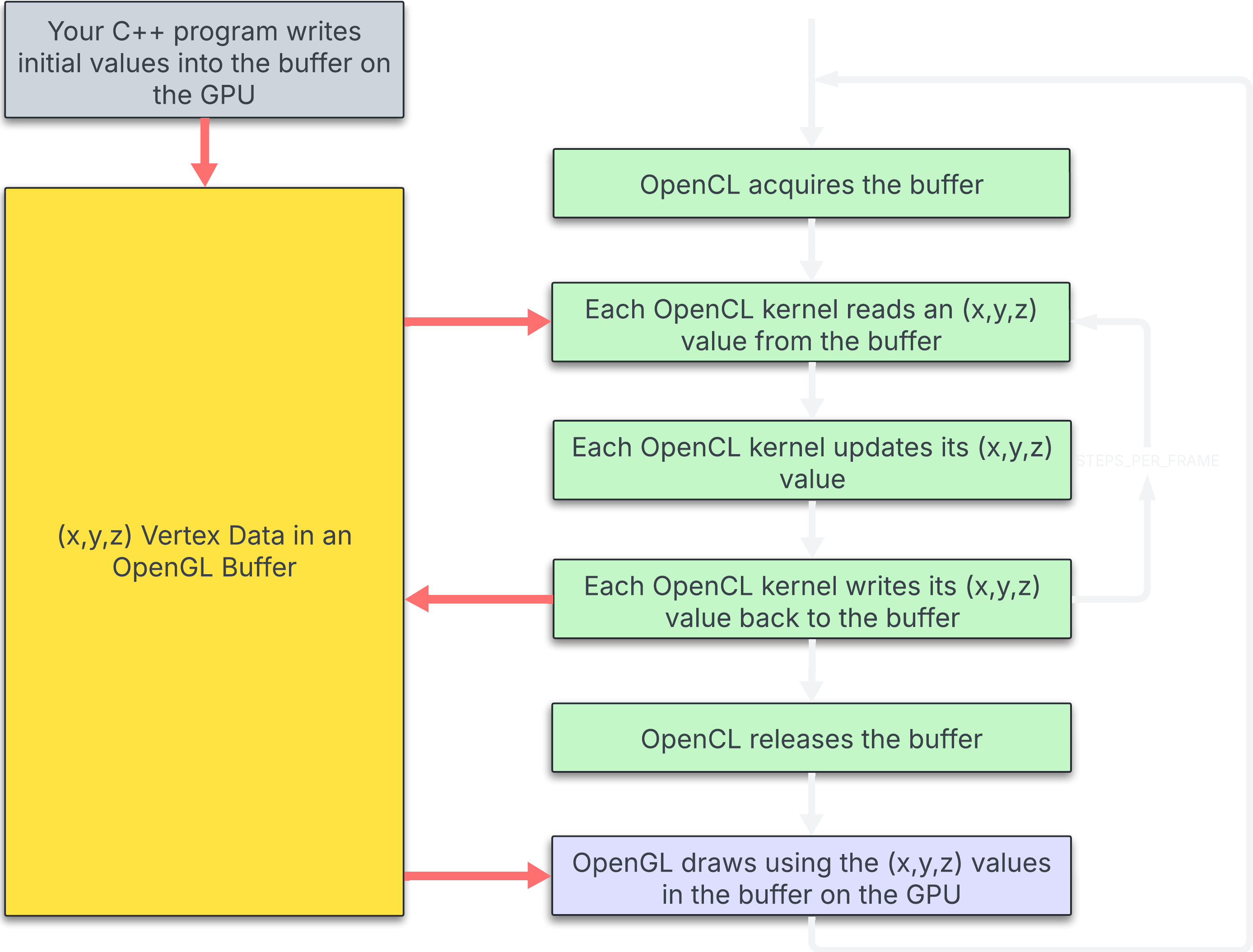
Looking at the graph, once we set up the data on the OpenGL side, OpenCL acquires it. As explained in the OpenCL/GL Interoperability notes, synchronization is required because only one can hold the buffer at a time. OpenCL runs a kernel that reads an x, y, and z value, updates it according to projectile motion laws, writes it back to the buffer, and releases it. OpenGL then draws the buffer, and the cycle repeats.
While this system works, it means only one physics update happens per visual frame. Each frame carries fixed overhead: synchronizing OpenGL and OpenCL, acquiring and releasing the buffer, and driver command submission. This overhead is paid once per frame regardless of how much compute work you do.
If you're locked to your monitor's refresh rate (let's assume 60Hz), you'll draw 60 frames per second, which is your framerate. But here's the catch: Just because you can only draw 60 frames per second doesn't mean you can only compute 60 times per second.
STEPS_PER_FRAME determines how many compute kernels are launched before drawing a frame. We want to know "How fast can my GPU update particles?" not "How many frames can I draw?" When STEPS_PER_FRAME is set higher than 1, you're running multiple physics updates per visual frame.
Think of your GPU like a delivery truck. Every frame is a "trip", and every kernel compute is a "package".
- Make 1 delivery per trip (
STEPS_PER_FRAME=1): You drive out, drop off one package, and drive all the way back. Most of the trip is overhead. Inefficient! - Make 10 deliveries per trip (
STEPS_PER_FRAME=10): You drive out once, hit 10 houses, then come back. The drive is the same cost, but you're doing 10× more useful work during it.
Your GPU has limits, so setting the value too high will hurt your framerate. Increasing STEPS_PER_FRAME amortizes the per-frame overhead across more physics updates, so the GPU spends a greater fraction of its time doing real work. Your goal is to find the value that stresses your GPU the most while maintaining fluid motion. An easy way is to increase the value until your FPS drops to around your monitor's refresh rate. Or just pick a really high value (e.g., 1024), and see what happens. You will be running tests with both STEPS_PER_FRAME = 1; and STEPS_PER_FRAME = ???;, where ??? is the value you chose.
When finding this value, test with your maximum particle count.
3. Add Additional Bumper Object
Your simulation must have at least two "bumpers" in it for the particles to bounce off of. Each bumper needs to be geometrically designed such that, given particles XYX, you can quickly tell if that particle is inside or outside the bumper. To get the bounce right, each bumper must know its outward-facing surface normal everywhere.
What's the easiest shape for a bumper? A sphere! In computer graphics, we love spheres as they are computationally "nice". It's fast and straightforward to tell if something is inside or outside of a sphere. It's just as straightforward to determine a normal vector for a point on the surface of a sphere.
It is OK to assume that the two bumpers are separate from each other; that is, a particle cannot collide with both at the same time.
Your OpenCL .cl program must also handle bounces from your (>=2) bumpers. Be sure to draw these bumpers in your .cpp program in InitLists() so that you can see where they are.
Warning
Don't forget to update the .cl kernel code with the same values you set in your .cpp code.
4. Implement Dynamic Color Changes
The sample OpenCL code does not retrieve the colors, modify them, or restore them. However, your .cl kernel needs to change the particles' colors dynamically. You could base this on position, velocity, time, bounce knowledge, etc. The way they change is up to you, but the color of each particle needs to change in some predictable way during the simulation.
I recommend reading Explaining the Kernel, as it explains the kernel code that you will be updating. Plus, it shows how the color type is defined and how color values are read from and written back to the global buffer.
OpenGL defines the red, green, and blue components of a color each as a floating-point value between 0.0 and 1.0
5. Test Performance
Vary the total number of particles from something small-ish (~1024) to something big-ish (~1024*1024) in some increments that will look good on the graph.
If you check the "show performance" box, you will see current, peak, and average measurements. Let the simulation run for a few seconds, and then write down your Average GigaParticles/Sec.
Are your particles moving too slow or too fast? Adjust the BASE_DT constant in the code. Larger values speed up movement, smaller values slow it down.
6. Show Results
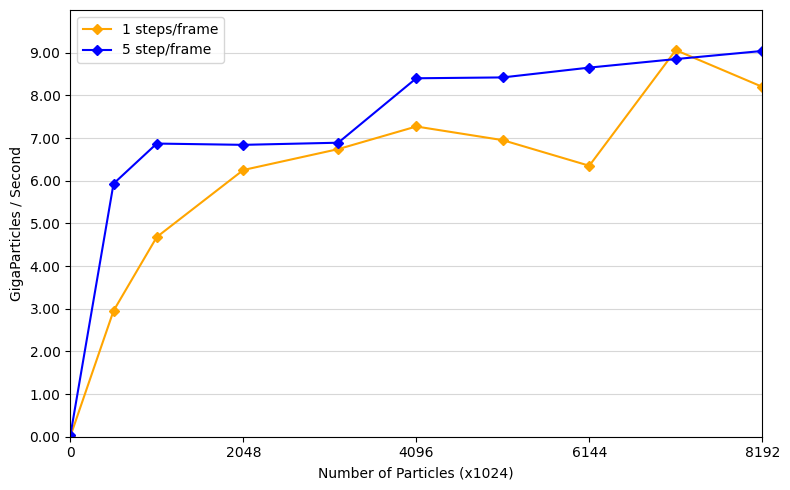
Create a table and a graph of Performance vs. Total Number of Particles. Test with at least five different particle counts, ranging from something small (~1024) to something large (~1024 × 8192). Run the full set of tests under both STEPS_PER_FRAME = 1; and STEPS_PER_FRAME = ???;, where ??? is the value you chose.
By increasing STEPS_PER_FRAME, we do more physics per frame, spending less time on per-frame overhead relative to useful work. The potential rising GigaParticles/sec score reflects the GPU staying busy rather than waiting on synchronization.
Example Graph
Want to make a graph with code?
I used Python Playground to make my graph. Here is the code I used if you want to do something similar. You might have to change the range and tick values to suit your results better.
import matplotlib.pyplot as plt
import numpy as np

# ─── FILL IN YOUR DATA HERE ───────────────────────────────────────────────────
PARTICLES_1     = [1, 512, 1024, 2048, 3172, 4096, 5120, 6144, 7168, 8192]  # x1024
GPS_1           = [0.008, 2.95, 4.68, 6.25, 6.74, 7.27, 6.95, 6.35, 9.06, 8.20]
STEPS_LABEL_1   = "1 steps/frame"

PARTICLES_2     = [1, 512, 1024, 2048, 3172, 4096, 5120, 6144, 7168, 8192]  # x1024
GPS_2           = [0.033, 5.93, 6.87, 6.84, 6.89, 8.40, 8.42, 8.65, 8.85, 9.04]
STEPS_LABEL_2   = "5 step/frame"
# ──────────────────────────────────────────────────────────────────────────────

fig, ax = plt.subplots(figsize=(8, 5))

ax.plot(PARTICLES_1, GPS_1, marker='D', markersize=5,
        color='orange', label=STEPS_LABEL_1)

ax.plot(PARTICLES_2, GPS_2, marker='D', markersize=5,
        color='blue', label=STEPS_LABEL_2)

ax.set_xlabel("Number of Particles (x1024)")
ax.set_ylabel("GigaParticles / Second")
ax.set_xlim(0, 8192)    # Bottom range
ax.set_ylim(0.0, 10.0)  # Left range
ax.set_xticks([0, 2048, 4096, 6144, 8192])                      # Bottom ticks
ax.set_yticks([round(v, 2) for v in np.arange(0.0, 10.0, 1.0)]) # Left ticks
ax.yaxis.set_major_formatter(plt.FormatStrFormatter('%.2f'))
ax.grid(axis='y', linestyle='-', alpha=0.5)
ax.legend()

plt.tight_layout()
plt.show()
7. Demonstrate your program in action
Make a video of your program in action and be sure it's Unlisted. You can use any video-capture tool you want. If you have never done this before, I recommend Kaltura, for which OSU has a site license for you to use. You can access the Kaltura noteset here. If you use Kaltura, be sure your video is set to Unlisted. If it isn't, then we won't be able to see it, and we can't grade your project.
Sites like YouTube also work. Just make sure your video is either public or unlisted, not private.
Tip
Copy and paste your video link into an incognito tab and see if it plays. If it does, you should be good to go.
8. Commentary in the PDF file
Your commentary PDF should include:
- A web link to the video showing your program in action -- be sure your video is Unlisted.
- What machine did you run this on?
- What predictable dynamic thing did you do with the particle colors? random changes are not good enough
- Include at least one screenshot of your project in action
- Show the table and graph.
- What patterns are you seeing in the performance curve?
- Why do you think the patterns look this way?
- What does that mean for the proper use of GPU parallel computing?
Tips
Explaining the Sample Code
Joe Parallel has already set up a complete OpenCL/OpenGL particle system for you. The sample code allocates the data, connects it to the GPU, talks to the OpenCL kernel each frame, and then draws the particles.
The Particle Data
Each particle has a position, a color, and a velocity, all stored as 4-component floats:
struct xyzw { float x, y, z, w; };   // positions and velocities
struct rgba { float r, g, b, a; };   // colors
Joe reuses xyzw for both positions and velocities (it is just four floats). The w in positions is the homogeneous coordinate (almost always 1.0). The a in colors is alpha (transparency), which is set but not used by the shaders right now.
Where the Data Lives
There are three main pieces of particle storage:
particle.posGL   // An OpenGL VBO for positions
particle.colorGL // An OpenGL VBO for colors
particle.velHost // A host-side array for velocities
particle.velCL   // A matching OpenCL buffer for velocities
The position and color VBOs are also turned into OpenCL buffers (particle.posCL, particle.colorCL) using clCreateFromGLBuffer. That means OpenCL and OpenGL share the same memory for positions and colors, so there is no copying back and forth.
How Particles Get Their Starting Values
The function ResetParticles() is Joe's “initial conditions” step. It:
- Maps the position VBO with
glMapBuffer, fills GPU memory directly with random(x,y,z)positions in a 3D box, and setsw = 1. - Maps the color VBO, fills GPU memory with random bright colors, and sets
a = 1. - Fills the host velocity array
particle.velHostwith random(vx, vy, vz)values, then usesclEnqueueWriteBufferto copy those velocities into the OpenCL bufferparticle.velCL.
At this point, all particles have a randomized position, color, and velocity, and both APIs agree on where that data lives.
How OpenCL and OpenGL Share the Work
Initialization in InitCL() does the heavy lifting Joe does not want you to worry about:
- Picks an OpenCL device and creates a context that can share with the current OpenGL context.
- Creates the OpenCL views of the OpenGL position and color VBOs with
clCreateFromGLBuffer. - Creates the pure-OpenCL velocity buffer, builds the
Particlekernel fromparticles.cl, and sets up the kernel arguments: position buffer, velocity buffer, color buffer, and the time stepdt.
After that, the compute side is ready to run; you do not need to change any of this setup to experiment with the kernel.
What Happens Each Frame
Every frame, Animate() runs the simulation step before anything gets drawn:
- Pause Check: If the app is paused, nothing happens.
- Give Buffers to OpenCL:
clEnqueueAcquireGLObjectstells OpenGL to stand back while OpenCL updates the shared position and color buffers. - Set the Time Step: A small
dtis computed (BASE_DT / STEPS_PER_FRAME) and passed as kernel argument 3. - Run the Kernel: The
Particlekernel is launchedSTEPS_PER_FRAMEtimes over allNUM_PARTICLES. Each work-item handles one particle and updates its position, velocity, and (optionally) color. - Give Buffers Back to OpenGL:
clEnqueueReleaseGLObjectshands the shared buffers back, andclFinishwaits for everything to complete.
By the time this function returns, the OpenGL VBOs contain the new particle positions and colors ready to be drawn.
How the Scene Gets Drawn
The Render() function handles all of the drawing:
- Sets up the camera and projection (perspective or orthographic).
- Draws the wireframe spheres that act as bumpers for the particles (the same spheres are defined in the OpenCL kernel for collision).
- Binds the particle VAO and calls
glDrawArrays(GL_POINTS, 0, NUM_PARTICLES)to draw every particle as a point, using the shared position and color data.s - Renders the ImGui UI and performance overlay on top.
So, by the time drawing happens, no CPU-side loops are needed to touch individual particles. Everything is done on the GPU.
Explaining the Kernel
Advancing a Particle by DT
In the sample code, Joe Parallel wanted to clean up the code by treating x, y, z positions and velocities as single variables instead of handling each component separately. To do this, he created custom types called point, vector, and color using typedef, all backed by OpenCL's float4 type. (OpenCL doesn't have a float3, so float4 is the next best option, the fourth component goes unused.) He also stored sphere definitions as a float4, packing the center coordinates and radius as x, y, z, r.
typedef float4 point;   // x, y, z, 1.
typedef float4 vector;  // vx, vy, vz, 0.
typedef float4 color;   // r, g, b, a
typedef float4 sphere;  // x, y, z, r

Spheres[0] = (sphere)(-100.0, -800.0, 0.0, 600.0);
Joe Parallel also stored the (x,y,z) acceleration of gravity in a float4:
const vector G = (vector)(0.0, -9.8, 0.0, 0.0);
Now, given a particle's position point p and a particle's velocity vector v, here is how you advance it one time step:
kernel
void
Particle( global point *dPobj, global vector *dVel, global color *dCobj )
{
int gid = get_global_id( 0 ); // particle number

point   p = dPobj[gid];
vector  v = dVel[gid];
color   c = dCobj[gid]; // (1)!

point  pp = p + v*DT + G*(point)(0.5 * DT * DT);    // p'
vector vp = v + G*DT;                               // v'

pp.w = 1.0;
vp.w = 0.0;
- This could be helpful

Bouncing is handled by changing the velocity vector according to the outward-facing surface normal of the bumper at the point right before an impact:
// Test against the first sphere here:
if(IsInsideSphere(pp, Spheres[0]))
{
  vp = BounceSphere(p, v, Spheres[0]);
  pp = p + vp * DT + G * (point)(0.5 * DT * DT);
}
And then do this again for the second bumper object. Assigning the new positions and velocities back into the global buffers happens like this:
dPobj[gid] = pp;
dVel[gid]  = vp;
dCobj[gid] = ????;  // Some change in color based on something
                    // happening in the simulation (1)
- This could also be helpful

Some utility functions you might find helpful:
| particles.cl | |
|---|---|
11 12 13 14 15 16 17 18 | |
| particles.cl | |
|---|---|
20 21 22 23 24 25 26 | |
| particles.cl | |
|---|---|
28 29 30 31 32 | |
Getting low GigaParticles / Second?
If your GigaParticles per Second are noticeably lower than Joe Graphics' results, that's completely normal, especially on a laptop. For example, a MacBook Air M4 will typically only hit around ~1.3 GigaParticles/Second with one million particles, and it'll be even lower without a dedicated GPU.
A good first step is to double-check that LOCAL_SIZE and STEPS_PER_FRAME are configured correctly. VSYNC can also drag your scores down a bit, particularly when STEPS_PER_FRAME is set to 1.
That said, if you're consistently under 1.0, you can switch the benchmark from GigaParticles/Second to MegaParticles/Second. In PerformanceOverlay(), change:
float gigaParticlesPerSec = (perf.elapsedTime > 0.0f) ? (float)NUM_PARTICLES / perf.elapsedTime / 1000000000.0f : 0.0f;
to:
float gigaParticlesPerSec = (perf.elapsedTime > 0.0f) ? (float)NUM_PARTICLES / perf.elapsedTime / 100000000.0f : 0.0f;
The only change is the divisor, which went from 1,000,000,000 down to 100,000,000.
Joe Graphics' Specs
The components used to produce the benchmark results shown above.
Ryzen 7 9800X3D @ 4.40GHz
RTX 3080
DDR5 6000 CL30
Determining Platform and Device Information
The sample code includes code from the printinfo program. This will show what OpenCL capabilities are on your system. The code will also attempt to pick the best OpenCL environment. Feel free to change this if you think it has picked the wrong one.
To enable printinfo, set PRINTINFO to true
Don't know your monitors refresh rate? Try enabling VSYNC.
To enable VSYNC, set VSYNC to true.
VSYNC sometimes locks to double your screen's refresh rate.
Grading
| Requirement | Points |
|---|---|
| Convincing particle motion | 20 |
| Bouncing from at least two bumpers | 20 |
| Predictable dynamic color changes (random changes are not good enough) | 30 |
| Performance table and graph | 20 |
| Commentary in the PDF file | 30 |
| Potential Total | 120 |
Success
The motion, bouncing, and colors of the particles need to be demonstrated via a video link. If it is a Kaltura video, be sure it has been set to Unlisted.